Is Learning Feasible?: Hoeffding Inequality

Learning Intuition

The goal of these notes is answering the question: Is Learning Feasible? To do that, we first developed an intuition and then use the Hoeffding Inequality to formarly explain our inution.

The learner $\mathcal{A}$, in principle, only have limited data (==training set==) to pindown the theorical entire target function $f(x)$. However, this limited data set could reveal enough information or not depending of the prespective (discrete or ==probabilitic==), and we will describe these prespectives later.

First, it's important to define what we understand for feasible learning. Our notion of learning in this context is the following:

==Learning:== A learner is learning if it is able to tell us __anything outside of training set ($\mathcal{T}$)__.
==Memorization:== A learner is only memorizing if it only knows the target $f$ for all points in our training set.

Discrete Perspective

==**Why learning something outside $\mathcal{T}$ is challenging in a discrete perspective?**==

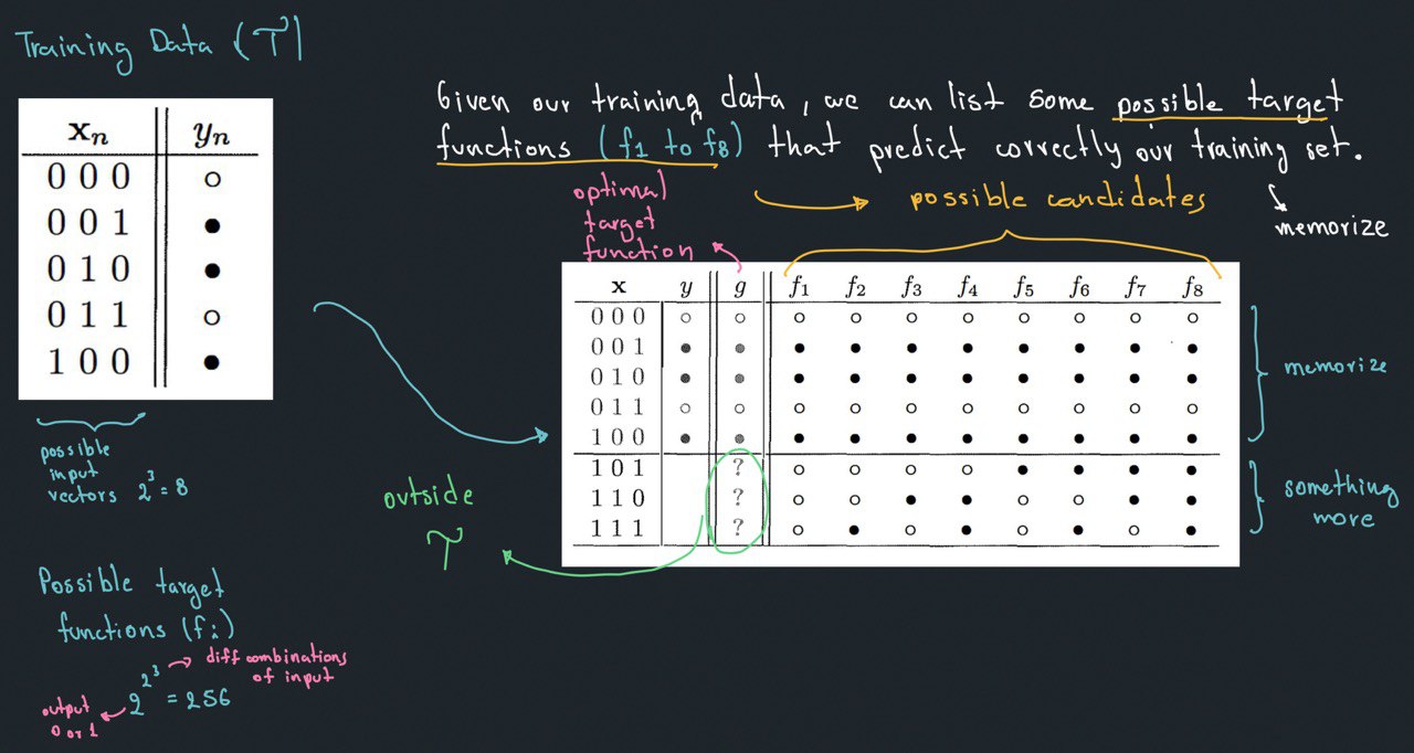
In a discrete prespective, we expect that our learner is able to learn all the in-samples and out-samples. However, that is not practically possible because our limited training set cannot tell us something ==concrete (or certain)== about something outside our training set.

Illustrated with an example, using the following training set, we are interested in learning an optimal function $g$, such that $g = f$; or in other words $g$ must be able to correctly predict **all** in-samples and out-samples.

Picking any of those candidates ($f_1, f_2, \cdots, f_8$) could be a possible optimal $g$ because they predict correctly our in-samples.

However, these candidates don't give us a concrete (certain) information outside the dataset (out-samples). Any possible value in ==**?**=='s can be acceptable in theory because we don't know what is actually happening outside the dataset.

Probabilistic Perpective

Nevertheless, although the discrete case is not possible, the training set can still give us a probabilitic approximation. We are able to ==infer== something outside $\mathcal{T}$ using only $\mathcal{T}$, but in a probabilitic way using __**Hoeffding Inequality**__.

Hoeffding Inequality

Hoeffding Inequality is a ==concentration inequality==, which provides an exponential bound on the probability that the ==sample mean== deviates significantly from the ==true expected value==.

Let $z_1, \cdots, z_N$ be random independent indentically distributed random variables, such that $0 \leq z_i \leq 1$.

where,

$\nu = \frac{1}{N}\sum^N_{i=1}z_i$ is the sample mean
$\mu = E_{z\sim p}[z]$ is the expected value (or population value)

==Important Takeways==

It is ==not a tight bound== because is bounded by 2, and probability can't be greater than 1.
The only quantity that is random is $\nu$ (it a random variable), $u$ is unknown but not random.
The size of the population (bin) doesn't matter. The population could be small or large, finite or infinite.
__**iid condition**__: The fact that the sample is iid draw from the population is a necessary condition to apply Hoeffding Inequality.

In the general case, we use a bound on $a_i \leq z_i \leq b_i$, where $a_i$ and $b_i$ are constant per each $z_i$. Then, the RHS exponent changes to

Intuitively, to understand the Hoeffding Inequality, thing about a bin with read and blue balls, and an iid sample from this bin. Then, by the law of large numbers, it makes sense that the mean sample $\nu$ can tell us something about the expected value (or population mean) $\mu$. Hoeffding Inequality only quantifies this behavior.

There are others takeways on $\epsilon$ and $N$, which are better explained when Hoeffning is applied to machine learning later.

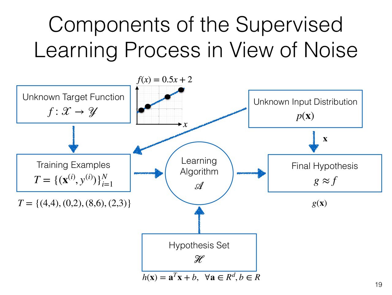
In order to use our Hoeffding Inequality in Machine Learning, we focused in the simple Supervised Learning Framework, where we try to predict $g: \mathcal{X} \rightarrow \mathcal{Y}$, such that $g$ approximates the true target function $f: \mathcal{X} \rightarrow \mathcal{Y}$.

In this framework, we can additionally distinguish in-sample and out-sample examples, which will be consider to calculate the errors:

in-sample examples are the training examples.
out-sample examples are ==**all**== the other examples that are not training examples, but belongs to $\mathcal{X}$.

Hoeffding in Machine Learning

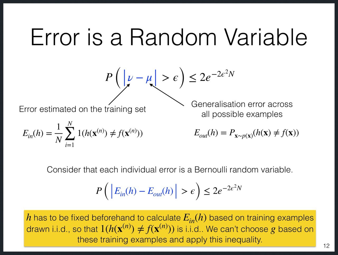
We can replace the respective sample mean and expected value from Hoeffding Inequality with our equivalence in Machine Learning, where

==$\nu = E_{in}$== is our in-sample error (or ==training error==).

It is our ==random variable== because it depends on a training set.
We can calculate this error because we know $f(x^{(i)})$ (our label from training set).

==$\mu = E_{out}$== is our out-sample error (or ==generalization error==) calculated across all possible examples.

It is unknown but not random.
We can't calculate it because we don't known $f(x)$

We can notice that using $E_{in}$ (or sample mean) tell us something about our $E_{out}$ (or expected value). Specifically, it tell us the our training error $E_{in}$ can approximate our $E_{out}$

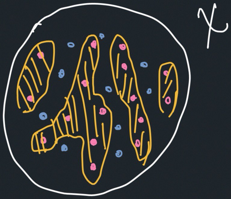
Notice $E_{out}$ is represented with a probability mass distribution where the points are $h(x) \neq f(x)$. In other words, all those points that produces wrong classification given a hypothesis $h$.

Intuitively, it's similar to the proportion of red balls in our bin example, but we now are dealing with a distribution.

NOTE: Although our $E_out$ is represented by a mass distribution, this distribution is derived from the expected value. In the ipad, I have an example of a derivation considering a binary classification problem.

Problem: No iid examples

In other words and to understand it better

In order to use the Hoeffding inequality, we have to **guarantee that the sample is drawn iid**.
However, in the Supervised Learning framework, we first choose $g$ using our training set.

If we train our model, find a $g$, fix that ==$g$==, and finally calculate $E_{in}(g)$. This error will not be calculated on iid examples anymore because the error is indirectly influenced by $g$ which was found using the same training set. Then, Hoeffding is invalid, and we need to come up with other bound.

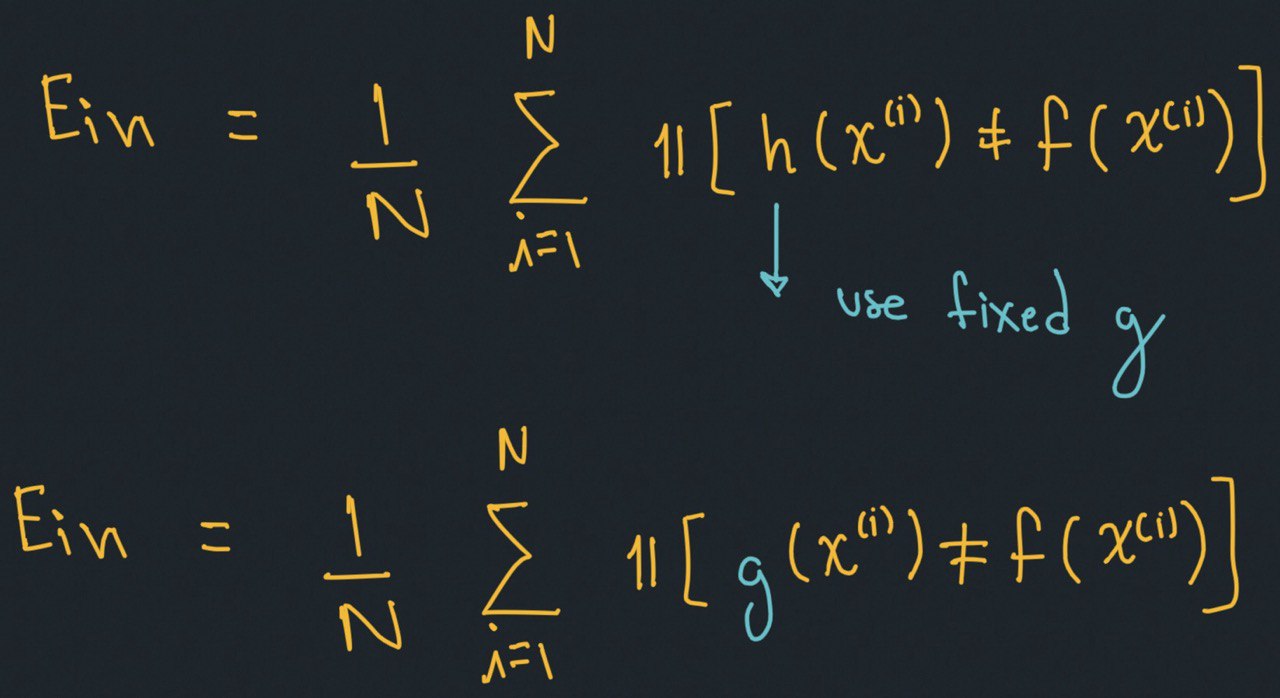
We can notice this problem is also visible in the definition of the in-sample error:

if we use a fixed ==$g$== the whole calculation is not iid anymore because the indicator function is going to use the final hypothesis $g$ to count the number of miss-classifications.

Solution: Uniform Hoeffding Inequality

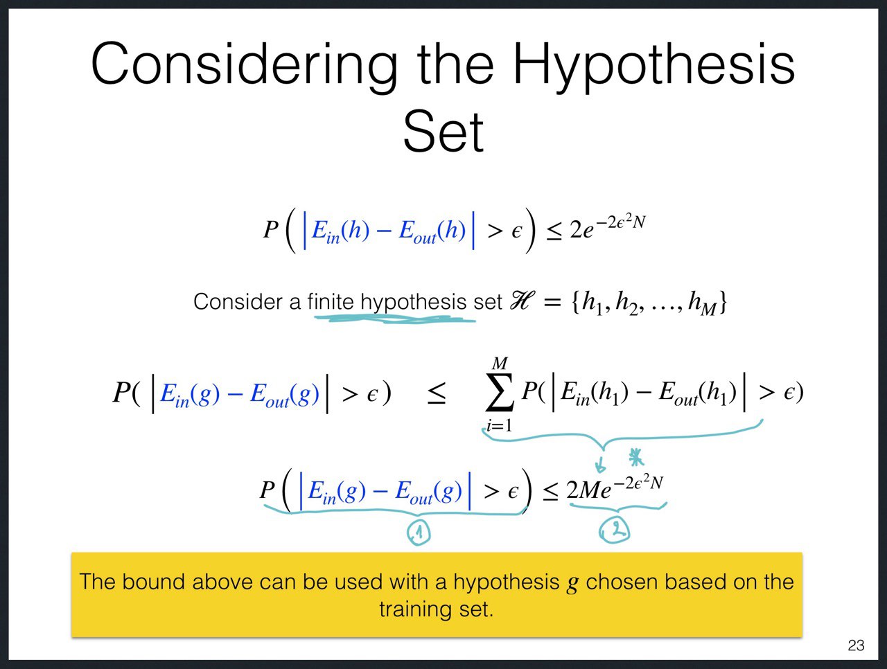
The way to solve this problem is to bound $P(|E_{in}(g) - E_{out}(g)| > \epsilon)$ in a way that doesn't depend on which $g$ the learning algorithm picks.

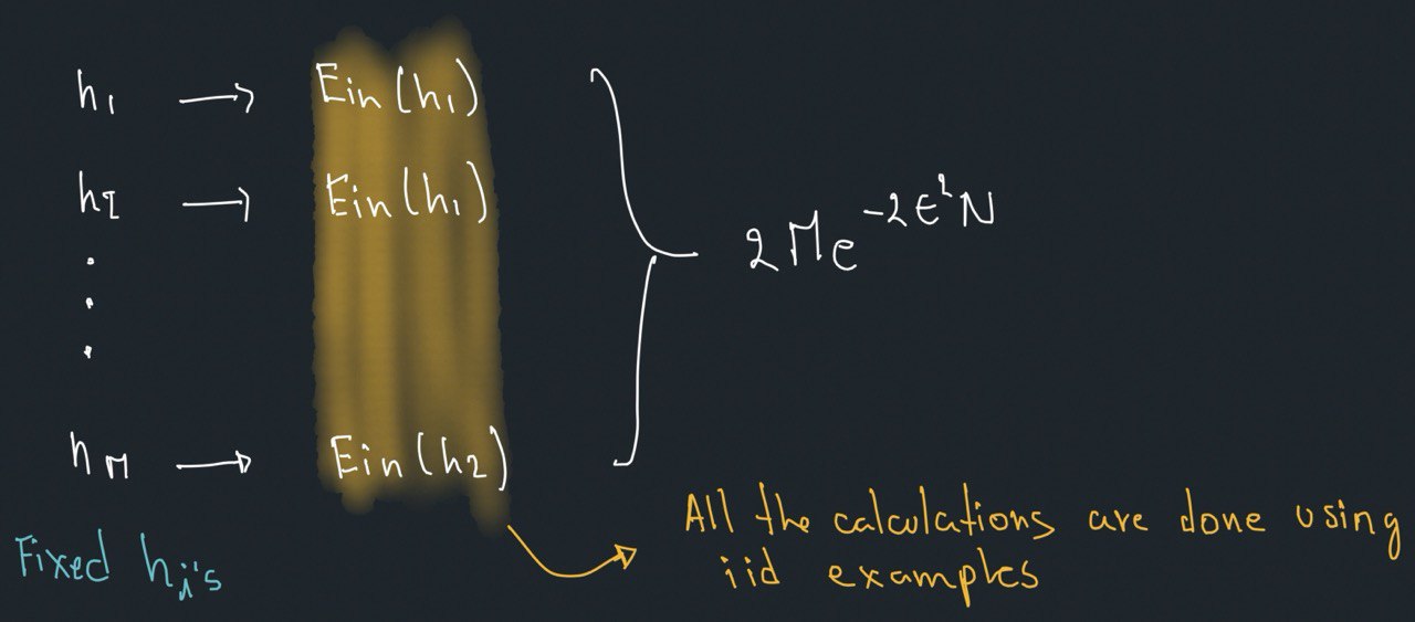
This result, also called __Uniform Hoeffding Inequality, is an overestimation__ of the LHS probability. It because as we can see in ==*==, we are taking into account all the fixed $h_i$'s. With this bound, intuiively, we are trying to simultaneously approximate the LHS with all the RHS corresponding to each $h_i$, which in some situations is not the best we can do, but for now it's great.

In this way, the new bound show us two things:

Our LHS comes from picking $g$ after training, normally as
But our RHS takes into account the whole hypothesis set, where it is guaranteed to draw iid examples to calculate each $E_{in}(h_i)$

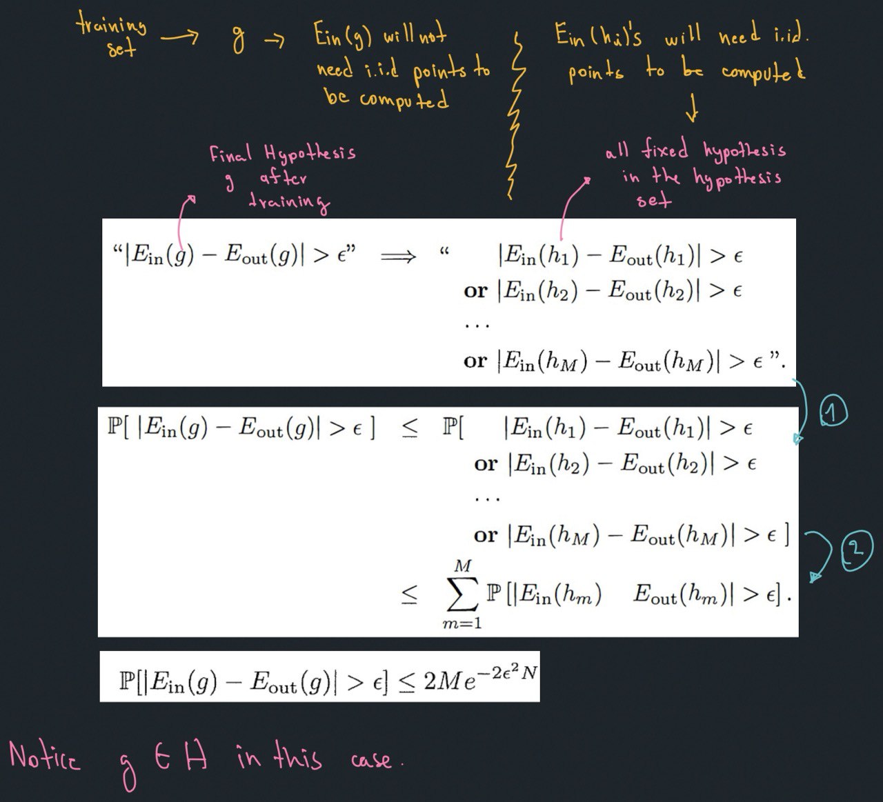
The whole derivation of this bound is below and we us two basic rules in probability

if $\mathcal{B}_1 \Rightarrow \mathcal{B}_2$, then $P(\mathcal{B}_1) \leq P(\mathcal{B}_2)$
__Union Bound__: $$P(\mathcal{B}_1 \text{or} \cdots \text{or} \mathcal{B}_M) \leq \sum_{i=1}^{M} P(\mathcal{B}_i)$$

Still idd condition

**IMPORTANT**

However, it stil important to assume the iid condition to use this bound:

==**When using $g$ to approximate $f:\mathcal{X} \rightarrow \mathcal{Y}$**==

A training and test examples are draw iid from ==$p(x)$==.
A training and test examples are all coming from the same target function $f$.

**==When using $g$ to approximate $p(x|y)$==**

Training and test examples are draw iid from ==$p(x,y)$==.

--I think we still need the iid condition because in some way we still need to guarantee that the RHS is calculated iid examples--

Note these conditions coincide with the supervised learning framework conditions

Conclusions

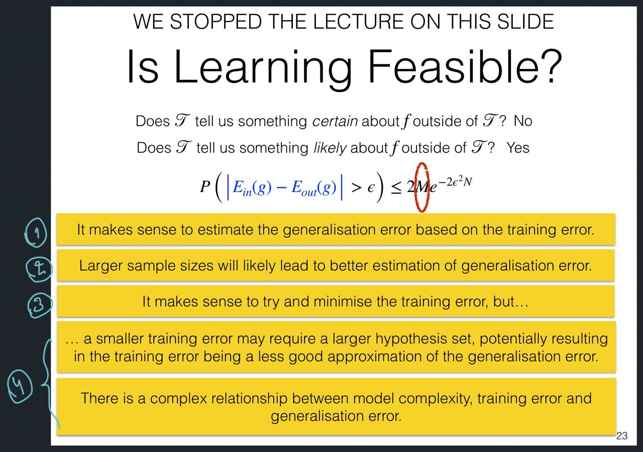
The training set $\mathcal{T}$ can only tell us something ==likely== about $f$ outside $\mathcal{T}$.

**==$\uparrow \epsilon \Rightarrow$==** $\downarrow \text{RHS} \Rightarrow$ $\downarrow$ probable that the difference $|E_{in}(g) - E_{out}(g)|$ was too high

$\Rightarrow$ it's more probable that those erros are close. Then, $E_{in}$ is a good estimate of $E_{out}$
**==$\uparrow N \Rightarrow$==** $\downarrow \text{RHS} \Rightarrow$ $\downarrow$ probable that the difference $|E_{in}(g) - E_{out}(g)|$ was too high

$\Rightarrow$ it's more probable that those erros are close. Then, $E_{in}$ is a good estimate of $E_{out}$
The third option is concluded by two previous ones.
There exists a __Trade-off between $M$, $E_{in}$, and $E_{out}$__

Trade-off between $M$, $E_{in}$, and $E_{out}$

By focusing in the complex relation that exists between $M$, $E_{in}$, and $E_{out}$, we can split the learning in two central questions:

can we make sure that $E_{out}(g)$ is close enough to $E_{in}(g)$
can we make $E_{in}(g)$ small enough?

Then, using the right $M$ (or $\mathcal{H}$) is important.

We will start to handle this trade-off later by changing our notion of model complexity using VC dimension.